Impact Demagnetization
MOTIVATION — Previous works calculate shock pressures from an impact without simulation tools like iSALE [1-3]. However, I personally found the explanation of methods to be very difficult to follow and contradictory in some places.
This document offers a simplified explanation/overview which a beginner could follow. See the original works for underlying citations and further explanations.
[1] Observed Crater Diameter Radius of Projectile
The Holsapple [1993] scaling relationship is
where:
- \(D_o\) — Observed crater diameter.
- Note: this is the only crater-dependent input for our calculation (not counting crustal density at that location).
- \(D_*\) — Transition diameter from simple to complex crater.
- Assumed 7km for Mars (Melosh, 1989).
- \(D_{tr}\) — Transient crater diameter.
From this, we can use the Schmidt and Housen [1987] relationship
where:
- \(v_{\text{proj}}\) — Projectile velocity.
- The majority of impact craters on Mars are formed by heliocentric projectiles with velocity 8-12 km/s (Neukum & Wise, 1976).
- \(g\) — Surface gravity of Mars.
- \(3.72076 \ \text{m} / \text{s}^2\)
- \(E_{\text{proj}}\) — Kinetic energy of projectile.
Now assume the projectile is spherical and composed of basalts. This lets us write out a few trivial relations:
- \(\rho_{\text{proj}} = 2,900 \ \text{kg} / \text{m}^3\)
- \(V_{\text{proj}} = \tfrac{4}{3} \pi r_{\text{proj}}^2\)
- \(E_{\text{proj}} = \tfrac{1}{2} M_{\text{proj}} v_{\text{proj}}^2\)
We combine all of these through \(\rho_{\text{proj}} = M_{\text{proj}} / V_{\text{proj}}\) and solve for the radius of the projectile to find:
[2] Shock Wave Pressures
[2.1] Generalized Hugoniot Equation
Consider the momentum jump condition from the Rankine-Hugoniot relations
where:
- \(P\) — Pressure behind the shock front (compressed region).
- \(P_0\) — Pressure ahead of the shock front (unshocked region), i.e. ambient/initial pressure.
- In this case, \(P_0\) is atmospheric pressure which is negligible.
- \(\rho_{\text{crust}}\) — Density of the target material, i.e. Martian crust.
- \(u_{sw}\) — Shock wave velocity, the speed at which the shock front propagates through the material.
- \(u_p\) — Particle velocity, the speed at which particles in the material move due to the passage of the shock wave.
Most materials exhibit a linear relationship between shock wave velocity and particle velocity (up to moderate pressures arounda few hundred GPa) according to laboratory experiments, modeled as
where:
- \(C\) — Represents the bulk sound speed (i.e. speed at which small-amplitude sound waves travel through the material under uncompressed/ambient conditions).
- Previous works give a wide range of values (\(2.6\), \(3\), and \(3.5\) \(\text{km} / \text{s}\)), some higher (?).
- The pressures we're interested in are about less than or equal to the Hugoniot elastic limit (the point where a material transitions from a purely elastic state to an elastic-plastic state), so we use this constant to model the propogation of shock waves for the entirety of this work.
- \(S\) — Characterizes the compressibility of the material under shock loading (higher values correspond to a material that is harder to compress at high pressures relative to its ambient compressibility).
- Previous works agree around \(1.5\).
Combining this with the Hugoniot equation, the total shock pressure at some point in the Crust is given by:
The primary source of depth-based variations in shock pressure is due to variations in particle velocity (\(u_p\)), which is discussed next.
[2.2] Direct Shock Pressure (i.e. Adding Depth Dependence)
[2.2.1] Near-shock
Previous impact simulation work shows that upon contact and compression, the initial convergence of shock waves creates a region of nearly uniform shock pressures known as the "isobaric core" (denoted "IC"). The volume of this region is roughly proportional to the dimensions of the projectile if it were completely buried (see fig. 1 in a later section for a basic diagram). We model this with:
where:
- \(r\) — Distance from the center of the isobaric core.
- \(R_{IC}\) — Radius of the IC.
- As previously explained, we assume \(R_{IC} \approx r_{\text{proj}}\) (for reference, some works say \(R_{IC} \approx 0.7 \cdot r_{\text{proj}}\); we assume they're the same size, it doesn't make a huge difference).
- \(u_{IC}\) — Particle velocity in the isobaric core.
- When the impactor and target have similar mechanical properties, the particle velocity is about half the impactor velocity, i.e. \(u_{IC} = \tfrac{1}{2} v_{\text{proj}}\).
[2.2.2] Far-shock
Outside the IC, the particle velocity decreases with distance according to a power law
where:
- \(n\) — Exponential decay constant.
- This varies widely between works. Melosh 1989 uses a constant \(n=1.87\), while Mitani 2003 uses variable \(n\) for different pressure regions. We use the former for our purposes ('intermediate' impacts where \(D_o < 500 \ \text{km}\), and we're only concerned about furthest demagnetization extent).
Many works approximate pressure decay using a power law (i.e., replacing \(u_{IC}\) with \(P_{IC}\)). However, the earliest reference I found attributes this decay to particle velocity instead (see page 18 of Perret & Bass, 1975 [doi]), with the pressure-based version being an approximation. This likely makes little difference, but it's worth noting.
[2.2.3] Putting it all Together
Substitute these \(u_p(r)\) into equation 6 to find pressure from the initial shock wave as a function of distance from the center of the isobaric core. This is denoted \(P_{\text{direct}}(r)\), since we apply some corrections for reflected waves in the next section.
For convenience, here's the full equation in terms of known values, although it may not render correctly based on where you're viewing this.
[2.3] Reflected Shock Wave Correction (Surface Boundary Condition)
During an impact, the induced pressure at the surface must drop to zero. This causes the shock wave to reflect, generating a rarefaction wave that travels back and interacts with the initial shock wave. If the rarefaction wave arrives before the peak pressure is reached (this period is known as the "rise time"), it can interfere with the buildup of the pressure wave and reduce the peak pressure achieved. See figure 1 below for a basic diagram.
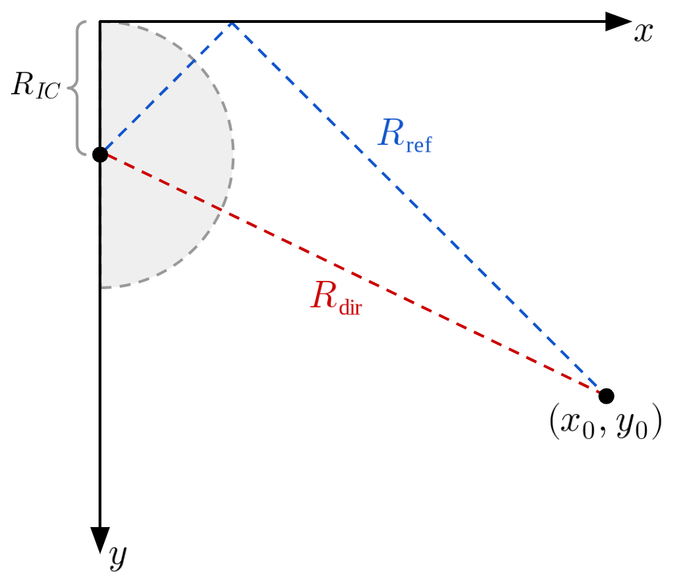
Figure 1: Path of direct and reflected shock waves to a given point.
To calculate this reduction, we begin by inferring some basic geometric relationships,
where:
- \(R_{\text{dir}}, R_{\text{ref}}\) — Distances traveled by the direct and reflected waves respectively.
- \(x,y\) — Horizontal and vertical distances from the impact point respectively.
At a given point, the difference in time between the arrival of the direct and reflected pressure waves is denoted:
whereas the rise time (the time it takes for the impact to reach peak pressure) is:
As before, the shock pressure is unaffected when \(\Delta t \geq \tau_{\text{rise}}\). However, when \(\Delta t < \tau_{\text{rise}}\), we reduce the direct pressure by the reflected wave attenuated by the additional distance traveled. Putting everything together, the effective subsurface shock pressure is given by:
References:
- [1] Mohit & Arkani-Hamed 2003
- https://files.catbox.moe/kbrqh9.pdf
- [2] Shahnas & Arkani-Hamed 2007
- https://files.catbox.moe/bqeh07.pdf
- [3] Melosh 2011
- https://sseh.uchicago.edu/doc/Melosh_ch_6.pdf